Introducing OpenFOAM
Choosing a CFD program can be a challenging and sometimes confusing task. There are many options to choose from, including common commercial codes such as ANSYS Fluent and Siemens Star-CCM++. Commercial CFD codes typically come with a simple user interface and plenty of documentation provided by the software vendor. However, commercial CFD software also requires expensive licensing fees that can make these options inaccessible, especially for smaller companies or those that can only make use of the software on an occasional basis. Even for heavy CFD users, the licensing fees can start to become out of control if they want to run massively parallel jobs on high-performance computing clusters, since additional fees typically need to be paid for the ability to run parallel jobs. For advanced CFD users it often becomes necessary to implement customized models. While commercial CFD codes do provide some ways to implement customizations, they are limited to specific parts of the code where the developer allows the user to add new functionality.
An alternative that has been steadily growing in popularity is an open-source code called OpenFOAM. Because of its open-source license, OpenFOAM is free to use by anyone, without the need to pay licensing fees, for any number of parallel tasks. It also provides full access to the source code so that any possible customization can be made by a qualified user. Despite these clear advantages, OpenFOAM does not have the simplified user interface that many commercial codes provide. The documentation is also much less plentiful, so the learning curve is significantly steeper. Our experience is that novice CFD users tend to gravitate more towards commercial codes, since they can get up and running faster. However, the simplicity of commercial codes can be misleading, where the user is able to obtain a solution, but has made critical errors in its setup. As a company, Maple Key Labs uses OpenFOAM for its CFD work. This allows us to develop customized models to solve the challenging problems given by our clients, while also offering them a cost advantage.
This blog article is intended for those readers who are interested in using OpenFOAM and want to learn more about the basics of how to use the program. In particular, this article describes the basic structure of an OpenFOAM case.
Directory Structure
Every OpenFOAM case consists of a directory structure containing specific files that are required to run the simulation. OpenFOAM is not just one solver, rather it contains many solvers developed from a common set of libraries. Therefore additional files may be required by some solvers and not for others. This article focuses specifically on the directories and files that are required for all solvers. A sample directory layout for a solver that requires only pressure and velocity (e.g. an incompressible solver for laminar flow) is shown below:
0/
...U
...p
constant/
...polyMesh/
...transportProperties
...turbulenceProperties
system/
...controlDict
...fvSchemes
...fvSolution
Here, the entries with a trailing / are directories, while those without are plain text files.
The "time" Directories
The 0 Directory
The 0 directory is a special time directory that contains the initial condition(s) for the simulation. Inside of this directory there will be one text file for each field that is required for the particular solver executable that is being run (e.g. U for velocity, p for pressure, etc.). Each file contains four main sections, including the header section.
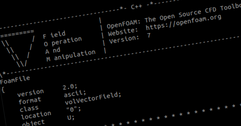
A header is included in each OpenFOAM file to give the parameters of the file, which can be checked by the solver prior to reading. Here is an example of the header section for the p file located in the 0 directory:
/*--------------------------------*- C++ -*----------------------------------*\
  =========                 |
  \\      /  F ield         | OpenFOAM: The Open Source CFD Toolbox
   \\    /   O peration     | Website:  https://openfoam.org
    \\  /    A nd           | Version:  7
     \\/     M anipulation  |
\*---------------------------------------------------------------------------*/
FoamFile
{
    version     2.0;
    format      ascii;
    class       volScalarField;
    location    "0";
    object      p;
}
// * * * * * * * * * * * * * * * * * * * * * * * * * * * * * * * * * * * * * //
The first 7 lines are comments, which are included by convention, but are not strictly necessary. All OpenFOAM files can be commented using C++ syntax. The entries inside of the FoamFile{...} section indicate several properties of the file that may be checked by the solver prior to reading the field. One item to note is that the version field refers to the I/O format, not the solver version. The I/O version is currently 2.0 and has remained as such for quite some time. After the FoamFile{...} section, there is one more commented line before the main content of the file begins. This line is included purely for decoration and is not technically required.
After the header, the next section indicates the dimensions of the field that is specified by the given file. Correct specification of dimensions is important in OpenFOAM, since the code will check that dimensions are consistent when performing arithmetic operations, and will return an error if dimensions are incompatible. An example of the dimension specification section for the p field is as follows:
dimensions [0 2 -2 0 0 0 0];While this statement may initially appear cryptic, it should be noted that dimensions in OpenFOAM are specified using an array of 7 integers, where each integer represents the exponent on one of the fundamental base units. The 7 base units are:
| Position | Dimension | SI Unit |
|---|---|---|
| 1 | Mass | Kilogram (kg) |
| 2 | Length | Metre (m) |
| 3 | Time | Second (s) |
| 4 | Temperature | Kelvin (K) |
| 5 | Quantity | Mole (mol) |
| 6 | Current | Ampere (A) |
| 7 | Luminous intensity | Candela (cd) |
Therefore, according to this table, the dimensions of pressure are m^2/s^2. Note that most of the incompressible solvers in OpenFOAM divide the momentum equation by density, such that the pressure field is actually p/\rho, which indeed has dimensions of m^2/s^2.
Following the specification of the dimensions is the specification of the initial value for the internal field, which is normally a statement of the form:
internalField uniform 0;This example would set the value of the field to a uniform value of 0 at every cell within the domain (taking the units that are specified by the dimensions keyword). This type of statement would apply to any scalar field. For a vector field (e.g. velocity), the statement would look something like this:
internalField uniform (0 0 0);In this case, the value in each cell is still set to a uniform value, but now contains a separate value for each component of the vector. It is also possible to specify n-dimensional tensors in a similar manner, where each component must be specified individually. Normally, the keyword uniform is used when setting the initial values, but it is also possible to specify a separate value for each cell using the keyword nonuniform. Normally this is not done manually, but will come up when using data from a previous simulation as the initial condition for a subsequent one.
The final section of the file includes the specification of the boundary conditions, using the keyword boundaryField. This keyword is followed by a set of braces ({...}) that contain an entry for every "boundary patch" that is contained in the mesh for the particular case. In OpenFOAM, a boundary patch is simply a named collection of faces that lie on the exterior boundary of the domain. An example is as follows:
boundaryField
{
    outlet
    {
        type            fixedValue;
        value           uniform 0;
    }
    ...
}
Here, the ... characters would be replaced with the remaining boundary conditions. The name outlet in this case would correspond with the exact name of a boundary patch that is specified in the mesh. Every boundary condition must specify a type and most require a value. Different boundary conditions may require additional keywords to be specified. This example is one of the simplest boundary conditions, called fixedValue, which in this case will set the value on all faces of the patch outlet to a uniform value of 0.
The set of valid boundary conditions is dependent on the particular solver being used and the type of field being set (i.e. not all boundary conditions are applicable to both velocity and pressure fields). One easy way to find out the set of valid boundary conditions is to attempt to run the case with an invalid type (the "banana test" as it has become known in the OpenFOAM community). If the boundary condition type is invalid, the OpenFOAM solver will stop running the case and provide a list of all the valid boundary conditions. For example, if the type is specified as banana for the velocity field in the pimpleFoam solver, the following will be output:
--> FOAM FATAL IO ERROR:
Unknown patchField type banana for patch type patch

Valid patchField types are :

85
(
SRFFreestreamVelocity
SRFVelocity
SRFWallVelocity
...
wedge
zeroGradient
)
Here, the ... is used in place of the full list of valid boundary conditions, since there are 85 valid boundary condition types for this particular solver and field type. Note that there is nothing special about the word banana; any invalid word would produce the same result.
The Remaining Time Directories
In addition to the 0 directory, the solver will output additional time directories that correspond to the solution fields at those particular times. The name of these directories will be the numerical value of the simulation time for which the solution is output, for example 0.001 or 10. The frequency of output is controlled by the controlDict file, which will be discussed later. In general, you will want to avoid writing these time directories too frequently to avoid spending too much time writing to disk and taking up a lot of hard drive space.
The constant Directory
The constant directory contains files that are related to the physics of the problem, including the mesh and any physical properties that are required for the solver. It does not contain information about how to run the simulation (e.g. timestep, linear solvers, etc.). Anything related to running the simulation is contained within the system directory, which will be discussed in the next section.
The constant directory will always contain a subdirectory called polyMesh which contains a number of files related to the mesh for the case. These files are not written by the user but created by a meshing utility. The most basic meshing tool that comes with OpenFOAM is blockMesh, which is suitable for simple cases, but becomes difficult to use for more complicated geometries. OpenFOAM also includes a tool called snappyHexMesh, which can create meshes for objects with triangulated surfaces. Further, external meshing software can be used. Many meshing software packages can directly export the necessary files for the polyMesh directory. For those that cannot, OpenFOAM includes several utilities to convert mesh formats (e.g. the ANSYS .msh format).
The constant directory normally contains a number of other files that are solver-specific. Typically, there will be a file called transportProperties that specifies the necessary physical properties. As an example, the following would be contained in the transportProperties file for the pimpleFoam solver (neglecting the file header):
transportModel  Newtonian;
nu              [0 2 -1 0 0 0 0] 1.0e-06;
Here, the file specifies that the fluid is to be treated as Newtonian, with a specified kinematic viscosity. As described previously, the integers in square brackets indicate the units of the quantity. The name nu is specified by the solver; if a value with this name is not found, then the solver will fail. Like the boundary conditions, inputting an invalid option for transportModel will get the solver to print the list of available options, in this case:
7
(
BirdCarreau
Casson
CrossPowerLaw
HerschelBulkley
Newtonian
powerLaw
strainRateFunction
)
Each of these models can then be looked up in the OpenFOAM documentation to determine the required parameters.
Another common file that can be found in the constant directory is the turbulenceProperties file, which specifies the turbulence model that should be used and its associated parameters. Note that even in the case of a laminar flow, the turbulenceProperties file is required, but the keyword simulationType would be set to laminar.
As mentioned, additional files may be required, depending on the solver being used.
The system Directory
The system directory contains files related to how the simulation is to be solved. There are three files that are mandatory: fvSchemes, fvSolution, and controlDict. Additional files may be included as well that are not mandatory. One example would be if the blockMesh tool is being used to prepare the mesh, then a blockMeshDict file would be required to specify the parameters of the mesh. Additional files may also be included to control runtime post-processing activities.
The fvSchemes file specifies all necessary information related to the discretization schemes for the finite volume method. It will normally specify the following information:
ddtSchemes: specifies how each equation is integrated with respect to timegradSchemes: specifies how the gradient of each field is calculateddivSchemes: specifies how divergence terms (e.g. convection term) are discretizedlaplacianSchemes: specifies how Laplacian terms (e.g. diffusion term) are discretizedinterpolationSchemes: specifies how interpolation from cell-centred values to face-centred values are computedsnGradSchemes: specifies how surface-normal gradient terms (e.g. heat flux terms) are discretized
A complete discussion of all of the schemes that can be specified for each of these items is beyond the scope of this article, however, many samples can be found in the provided OpenFOAM tutorial files (located in the directory given by the $FOAM_TUTORIALS environment variable).
The fvSolution file specifies how the discretized equations are to be solved. The solvers entry specifies the list of linear solvers that are used to solve each equation. An optional entry called relaxationFactors allows the user to set under-relaxation on a per-equation basis and to relax field variables between update steps. Most solvers also require a dictionary to specify solver-specific parameters, e.g. for PIMPLE-based solvers:
PIMPLE
{
    nNonOrthogonalCorrectors 1;
    nCorrectors              1;
    nOuterCorrectors         10;
    pRefCell                 0;
    pRefValue                0;
}
This sub-dictionary specifies a number of solver-specific correction parameters (i.e. nNonOrthogonalCorrectors, nCorrectors, and nOuterCorrectors) as well as parameters that allow the solver to fix the pressure at a specific point in the domain when none of the boundary conditions fix the pressure level (i.e. pRefCell and pRefValue). This is about the most basic PIMPLE sub-dictionary that can be specified. There are a number of additional parameters that can be specified to further control the behaviour of the solver.
Again, a complete discussion of all possible parameters that can be specified in fvSolution is beyond the scope of this article. The tutorial cases that come with the OpenFOAM installation are a good resource for sample files.
Finally, the controlDict file specifies how the solution should progress by specifying things like the timestep, how often to write solution data, as well as more advanced items such as function objects that should be executed at runtime. A basic controlDict file, neglecting the header, looks something like this:
application      pimpleFoam;
startFrom        latestTime;
startTime        0;
stopAt           endTime;
endTime          36000;
deltaT           300;
writeControl     runTime;
writeInterval    600;
purgeWrite       2;
writeFormat      ascii;
writePrecision   6;
writeCompression off;
timeFormat       general;
The most common parameters to adjust in the controlDict:
deltaT: specifies the timestep of the simulationendTime: specifies at what time to stop the simulation (assumingstopAtis set toendTime)writeInterval: specifies how often (in simulation time) to write output files (assumingwriteControlis set torunTime)purgeWrite: species how many timestep directories to keep; when running a simulation to steady-state, this allows intermediate timestep files to be deleted if not needed, while being able to access them while the simulation runs
Of course there are many other parameters that can be set in the controlDict, but these basic parameters are normally enough to get a simulation up and running.
How to Get Additional Support
There are a number of excellent resources available for learning OpenFOAM, including:
- The documentation website provided by CFD Direct (the organization largely responsible for development of the OpenFOAM.org branch of the code).
- The C++ source guide, which allows you to explore the code, including documentation that is automatically generated by the doxygen tool.
- The CFD Online OpenFOAM Forums, which is an excellent place to ask additional questions.
Maple Key Labs is also able to help you along your journey of learning OpenFOAM. We will continue to regularly post articles like this one, explaining different aspects of the code. The best way to stay up to date on the blog is to subscribe to our newsletter. We also offer one-on-one consultations with clients to assist with OpenFOAM model development. Navigate to the Contact Us page to request a consultation.
About the Author
Chris DeGroot, PhD, PEng, is the co-founder and CEO of Maple Key Labs. He is a leading figure in the promotion of CFD in Canada, having served on the Board of Directors of the CFD Society of Canada (CFDSC) for a number of years. Through his work with CFDSC, he served as Chair of the society's national conference in 2019, which was hosted in London, Ontario. He has been working in the field of CFD for more than 14 years, starting during his undergraduate studies. He earned his PhD in 2012 from Western University, after which he held a postdoctoral research fellowship at the University of Waterloo, in conjunction with ANSYS Canada. Starting in 2014 he began a journey to further develop the usage of CFD in the water industry through his work as a research scientist at Trojan Technologies. In 2016 he was appointed as Assistant Professor at Western University where he carried this interest through his research program to the present day. He is a current member of the International Water Association's (IWA) CFD Working Group and a member of the Water Environment Federation's Program Committee, which organizes the technical program of the WEFTEC conference. He is actively involved in the IWA's efforts to support Young Water Professionals (YWPs). In 2019 he co-Chaired the International YWP Conference in Toronto, Ontario and is currently the Treasurer of the IWA Canadian YWP Chapter.
Great explanation.
Pingback: Creating Block-Structured Meshes with blockMesh and ofblockmeshdicthelper – Maple Key Labs